Introduction to Python programming

A Brief Introduction

Python is a high-level programming language developed by a Dutch programmer Guido van Rossum in the 90’s (https://en.wikipedia.org/wiki/Python_(programming_language)). It is an interpreted language, which means the code does not need to be compiled prior to running it, like other languages such as C++ or Java. See here for more information: https://en.wikipedia.org/wiki/Interpreted_language

It is different from many other programming languages because of significane of white spaces. For example, the two following code snippets are interpreted differently, even though they have very similar code:

for i in range(1,10):
    print(i)

for i in range(1,10):
  print(i)

The difference is that the first one has 4 white spaces after code indentation, whereas the second one has only 2 white spaces. Python developers recommend the use of 4 white spaces to indent code for the code to be readable. See Python coding guidelines here: https://www.python.org/dev/peps/pep-0008/

It is easy to write any Python code but difficult to write beautiful code that is easy to read and easy to decipher/debug.

Today, you will be using both the jupyter-lab and terminal environment to write simple Python scripts that you can use to help you along with your projects. I will not be going over exhaustively what you can do with Python programming language but just brief introduction and I will be showing you important things you should know with regard to using Python for genomics work.

Basics

Python is already installed and running in your terminal environment because you have already installed Miniconda, which by default will install versions of Python you have downloaded. There is a significant difference between Python versions 2 and 3. They have made a lot of changes to code syntax between the two. For example, in Python 2 series, you can type like this to print something to screen:

print "Hello, World!"

But in Python 3 series, you need to type like this:

print("Hello, World")

This is just one of the examples. Since we are sticking to Python 3, we will need to use the code syntax as shown in the second example. In jupyter-lab, you can use code cells to start writing Python code right away. It works as a mini environment in which you can test things. For example, you can use it like a calculator.

print("Hello!")

Hello!

(134+8353-(2*20)) / 2

4223.5

Before we dive further into coding, a few important datatypes you need to know and remember in Python are listed below:

1. Booleans are either True or False.

2. Numbers can be integers (1 and 2), floats (1.1 and 1.2), fractions (1/2 and 2/3), or even complex numbers.

3. Strings are sequences of Unicode characters, e.g. an HTML document.

4. Bytes and byte arrays, e.g. a JPEG image file.

5. Lists are ordered sequences of values.

6. Tuples are ordered, immutable sequences of values.

7. Sets are unordered bags of values.

8. Dictionaries are unordered bags of key-value pairs.

For more details on the datatypes, refer to the tutorial here: https://diveintopython3.problemsolving.io/native-datatypes.html

The most common datatypes you will encounter in bioinformatics/genomics related context would be numbers, strings, lists, tuples, sets, and dictionaries.

Strings

Strings can be anything that will be treated as text. For example, a sentence like this:

"This is a string"

'This is a string'

When I just pasted a string in jupyter environment it just returns what’s being paste. However, you can put these strings into a variable. For example,

astring = "This is a string"

Now, you have a variable named astring. When you type this variable name in jupyter, you see this:

astring

'This is a string'

It just prints the string to screen. You can also turn anything into a string by using the str() function. For example, I have a bunch of numbers, which I want to treat it as text for some reason, I can do something like this:

s = str(12345)

Now, I have stored this “12345” into a variable named s. If you want to know what type of variable it is, you can type like this:

s.__class__

str

It returns a str, which means the variable s is a string. Once you have a string, you can do a lot of things with it. For example, you can split the string into individual words.

astring.split(" ")

['This', 'is', 'a', 'string']

In the example above, I have split the string in the variable astring into individual words and using space (” “) as a delimiter. You can also split without specifying the delimiter, in which case, the default action is to split by a white space.

astring.split()

['This', 'is', 'a', 'string']

Here, after you split the string into individual words, you will notice that you have each words contained within a single quote and all of them are in square brackets. What does this mean? This mean these are a list of words. In Python, anything contained within square brackets are treated as contents of a list. Let’s try to play around with this list.

Lists

alist = astring.split(" ")
alist[0]

'This'

What’s happening here? Here, I have stored the list produced as a result of string splittin function into a variable named alist. Then when you type alist[0], it subsets the first content of the list, which is the word 'This'. If you want to print the last item in the list, you can type:

alist[-1]

'string'

The “-1” in a list means you are accessing the last item within a list. If you want to print the items in a list one by one, you can type like this:

for i in alist:
    print(i)

This
is
a
string

Here, I am running a for loop to print the contents of a list one after another. In this example, the letter i is a variable that temporarily stores the contents of a list one by one. Then the print function prints the variable to screen in a loop.

Sets

Another useful datatype you can use is a set. Sets are a collection of unique values or items. For example, if you a list of items as shown below, you can turn into a set by typing the set() function.

another_list = ['A', 'B', 'B', 'C', 'D']
aset = set(another_list)

aset

{'A', 'B', 'C', 'D'}

As you can see, you have two instances of a 'B' and when you turn the list into a set, then only one of it is retained. Sets are usually contained in curly brackets { }. You can think of many scenarios in which sets can become useful; for example, getting unique names from a pool of names.

Dictionaries

Dictionaries are pairs of keys and values. As the name suggest, it behaves in the same way a dictionary would; it will explain meanings of a word, for example. Below is an example of a dictionary:

adict = {
    'A': 'x',
    'B': 'y',
    'C': 'z'
}

In this example, I have stored 3 keys named A, B, and C and their values x, y, and z. So when you want to look up what a key stored, you can type like this:

adict['A']

'x'

It prints the letter x which is stored as a value of the key A. You can only try to call key-value pairs that are present in this example dictionary. If you try to put a key that doesn’t exist, it will complain.

adict['D']

---------------------------------------------------------------------------
KeyError                                  Traceback (most recent call last)
<ipython-input-177-75bfd13c0a1b> in <module>
----> 1 adict['D']

KeyError: 'D'

As you can see, it gives you an error as Python could not find the key D in this dictionary.

To print all the keys in a dictionary, you can type like this:

adict.keys()

dict_keys(['A', 'B', 'C'])

And all the values in a dictionary can be printed like this:

adict.values()

dict_values(['x', 'y', 'z'])

The usefulness of dictionaries is probably not apparent at this point but as you grow your programming skill sets, you will start to realize it is a very useful feature of a programming language.

Tuples

Tuples are similar to lists but they are immutable, which means it stores values that cannot be changed and they are stored in parantheses ( ). Other datatypes such as lists and dictionaries are mutable, which means you can modify the contents after being created. Usually, I would store things in a tuple that I shouldn’t modify, for example, GPS coordinates. An example is shown below.

atuple = (1, 2, 3, 5)

atuple

(1, 2, 3, 5)

atuple[0] = 8

---------------------------------------------------------------------------
TypeError                                 Traceback (most recent call last)
<ipython-input-183-f087dd3c1bee> in <module>
----> 1 atuple[0] = 8

TypeError: 'tuple' object does not support item assignment

As you can see, it will not allow you to change the contents of it. A list, however, will allow you to do that. For example,

alist

['This', 'is', 'a', 'string']

alist[0] = 'Here'

alist

['Here', 'is', 'a', 'string']

As you can see here, I have replaced the first item in the alist variable with a string Here. So these few examples are to get you started with learning Python but you should explore outside of class to learn more in depth.

List comprehensions

Another very useful feature of Python is list comprehension. Let’s say you want to pull everything from one list that matches a criterion you provided and store it in another list, you can type like this:

blist = [i for i in alist if i == 'Here']

blist

['Here']

In this example, I have pull out the contents that match the string 'Here' into another list named blist. Let’s say if you want to pull out words that contain a letter s, you can type like this:

blist = [i for i in alist if 's' in i]

blist

['is', 'string']

Again, the usefulness of such functions may not be apparent to you at this time but eventually you will reach a point when features like these are indispensible to your coding workflow.

Useful Python libraries

Base python contains useful features that you can already start using but sometimes they come from other Python packages/libraries. Some of the important ones are listed below:

• pandas

• matplotlib

• numpy

• scipy

• seaborn

• biopython

Pandas

Pandas is a Python package oriented towards statistical analyses and provides a lot of useful features/functions that would otherwise take longer to code without it (see here: https://pandas.pydata.org/). For example, if you want to put a table into a dataframe, you can simply type something like this:

import pandas as pd
df = pd.read_csv("table.txt", sep="\t")

in this example, you are importing a “tab-delimited” (as indicated by the "\t") table into a dataframe named df. But before you can use Pandas and its features, you first need to import the library into your Python environment by typing import pandas as pd. This means you are importing the whole Pandas library and providing it a shortcut named pd. Let’s try and use Pandas here today. Download this file into a directory (maybe in a subfolder in your exercises folder): https://ftp.ncbi.nlm.nih.gov/genomes/ASSEMBLY_REPORTS/prokaryote_type_strain_report.txt

This file contains “type” strains of bacteria and archaea. Now, we will use Pandas to see what you can do with the table.

import numpy as np
np.__version__

'1.21.4'

import pandas as pd
df = pd.read_csv("prokaryote_type_strain_report.txt", sep="\t")

df.head()

	#scientific name	type materials and coidentical strains	has sequences from type material?	number of assemblies per taxon	number of assemblies from type materials per taxon	number of assemblies from type materials per species
0	'Burkholderia humi' Srinivasan et al. 2013	JCM 18069,KEMC 7302-068,Rs7	yes	0	0	0
1	'Lysobacter humi' Akter et al. 2016	CCTCC AB 2015292,KACC 18284,THG-PC4,culture-co...	yes	0	0	0
2	'Massilia aquatica' Lu et al. 2020	FT127W,GDMCC 1.1690,KACC 21482	yes	0	0	0
3	'Megasphaera vaginalis' Bordigoni et al. 2020	CSUR P4857,Marseille-P4857	yes	0	0	0
4	'Micromonospora endophytica' Thanaboripat et a...	BCC 67267,BCC<THA> 67267,DCWR9-8-2,NBRC ...	yes	0	0	0

df[df['#scientific name'].str.contains('Gloeobacter')]

	#scientific name	type materials and coidentical strains	has sequences from type material?	number of assemblies per taxon	number of assemblies from type materials per taxon	number of assemblies from type materials per species
8195	Gloeobacter kilaueensis	ATCC BAA-2537,BCCM ULC0316,CCAP 1431/1,JS1,cul...	yes	1	1	1
8196	Gloeobacter morelensis	MG652769	yes	1	1	1
8197	Gloeobacter violaceus	PCC 7421	yes	1	1	1

df.tail()

	#scientific name	type materials and coidentical strains	has sequences from type material?	number of assemblies per taxon	number of assemblies from type materials per taxon	number of assemblies from type materials per species
19403	[Ruminococcus] faecis	Eg2,JCM 15917,JCM:15917,KCTC 5757,KCTC:5757	yes	10	1	1
19404	[Ruminococcus] gnavus	ATCC 29149,ATCC:29149,VPI C7-9	yes	80	3	3
19405	[Ruminococcus] lactaris	ATCC 29176,ATCC:29176	yes	7	1	1
19406	[Ruminococcus] torques	ATCC 27756,ATCC:27756	yes	18	1	1
19407	[Scytonema hofmanni] UTEX B 1581	na	no	1	0	0

As you can see, I have just imported the table as a tab-delimited file, telling Pandas to put it into a dataframe named df. Once it’s put into a dataframe, it becomes easier to extract information from the table. For example, if you want to see all headers of the columns, type:

df.columns

Index(['#scientific name', 'type materials and coidentical strains',
       'has sequences from type material?', 'number of assemblies per taxon',
       'number of assemblies from type materials per taxon',
       'number of assemblies from type materials per species'],
      dtype='object')

This will list all the headers of all the columns in this dataframe. Let’s say you want to pull out all rows that contain Escherichia coli, you can type like this:

df[df['#scientific name'].str.contains('Escherichia')]

	#scientific name	type materials and coidentical strains	has sequences from type material?	number of assemblies per taxon	number of assemblies from type materials per taxon	number of assemblies from type materials per species
5808	Escherichia alba	na	no	1	0	0
5809	Escherichia albertii	Albert 19982,BCCM/LMG:20976,CCUG 46494,CCUG:46...	yes	224	1	1
5810	Escherichia coli	ATCC 11775,ATCC:11775,BCCM/LMG:2092,CCUG 24,CC...	yes	97292	5	5
5811	Escherichia fergusonii	ATCC 35469,ATCC:35469,BCCM/LMG:7866,CDC 0568-7...	yes	86	2	2
5812	Escherichia marmotae	CGMCC 1.12862,CGMCC:1.12862,DSM 28771,DSM:2877...	yes	35	2	2

By default, jupyter-lab will only print a few rows (perhaps up to 10 or 20). But when you write this code in a Python script, it will print everything to screen (if you run it in a terminal). Let’s count how many rows satisfy this criterion.

len(df[df['#scientific name'].str.contains('Escherichia')])

5

Looks like there are only 5 with the genus Escherichia. How about Salmonella?

len(df[df['#scientific name'].str.contains('Salmonella')])

10

df[df['#scientific name'].str.contains('Idiomarina')]

	#scientific name	type materials and coidentical strains	has sequences from type material?	number of assemblies per taxon	number of assemblies from type materials per taxon	number of assemblies from type materials per species
7752	Idiomarina abyssalis	ATCC BAA-312,ATCC:BAA-312,KMM 227,KMM:227,cult...	yes	13	2	2
7753	Idiomarina aestuarii	JCM 16344,JCM:16344,KCTC 22740,KCTC:22740,KYW314	yes	7	1	1
7754	Idiomarina andamanensis	BCCM/LMG:29773,JCM 31645,JCM:31645,LMG 29773,L...	yes	1	0	0
7755	Idiomarina aquatica	BCCM/LMG:27613,CCM 8471,CCM:8471,CECT 8360,CEC...	yes	2	1	1
7756	Idiomarina aquimaris	BCCM/LMG:25374,BCRC 80083,BCRC:80083,LMG 25374...	yes	1	1	1
7757	Idiomarina atlantica	G5_TVMV8_7,KCTC 42141,KCTC:42141,MCCC 1A10513,...	yes	1	1	1
7758	Idiomarina baltica	BCCM/LMG:21691,DSM 15154,DSM:15154,LMG 21691,L...	yes	3	1	1
7759	Idiomarina donghaiensis	908033,CGMCC 1.7284,CGMCC:1.7284,JCM 15533,JCM...	yes	2	2	2
7760	Idiomarina fontislapidosi	BCCM/LMG:22169,CECT 5859,CECT:5859,F23,LMG 221...	yes	2	2	2
7761	Idiomarina halophila	BH195,KACC 17610,KACC:17610,NCAIM B 02544,NCAI...	yes	1	1	1
7762	Idiomarina homiensis	DSM 17923,DSM:17923,KACC 11514,KACC:11514,PO-M2	yes	1	1	1
7763	Idiomarina indica	CGMCC 1.10824,CGMCC:1.10824,JCM 18138,JCM:1813...	yes	1	1	1
7764	Idiomarina insulisalsae	BCCM/LMG:23123,CIP 108836,CIP:108836,CVS-6,LMG...	yes	1	1	1
7765	Idiomarina loihiensis	ATCC BAA-735,ATCC:BAA-735,DSM 15497,DSM:15497,...	yes	6	1	1
7766	Idiomarina mangrovi	KCTC 62455,KCTC:62455,MCCC 1K03495,MCCC:1K0349...	yes	1	1	1
7767	Idiomarina marina	BCRC 17749,BCRC:17749,JCM 15083,JCM:15083,PIM1	yes	1	1	1
7768	Idiomarina maritima	908087,CGMCC 1.7285,CGMCC:1.7285,JCM 15534,JCM...	yes	2	1	1
7769	Idiomarina piscisalsi	NBRC 108617,NBRC:108617,TISTR 2054,TISTR:2054,...	yes	3	1	1
7770	Idiomarina planktonica	CGMCC 1.12458,CGMCC:1.12458,JCM 19263,JCM:1926...	yes	2	2	2
7771	Idiomarina ramblicola	BCCM/LMG:22170,CECT 5858,CECT:5858,LMG 22170,L...	yes	1	1	1
7772	Idiomarina salinarum	CCUG 54359,CCUG:54359,ISL-52,KCTC 12971,KCTC:1...	yes	2	2	2
7773	Idiomarina sediminum	BCCM/LMG:24046,CICC 10319,CICC:10319,DSM 21906...	yes	2	2	2
7774	Idiomarina seosinensis	CL-SP19,JCM 12526,JCM:12526,KCTC 12296,KCTC:12296	yes	1	1	1
7775	Idiomarina tainanensis	BCRC 17750,BCRC:17750,JCM 15084,JCM:15084,PIN1	yes	3	1	1
7776	Idiomarina taiwanensis	BCRC 17465,BCRC:17465,JCM 13360,JCM:13360,PIT1	yes	1	1	1
7777	Idiomarina tyrosinivorans	BCRC 80745,BCRC:80745,CC-PW-9,JCM 19757,JCM:19757	yes	1	1	1
7778	Idiomarina woesei	BCCM/LMG:27903,DSM 27808,DSM:27808,JCM 19499,J...	yes	2	2	2
7779	Idiomarina xiamenensis	10-D-4,BCCM/LMG:25227,CCTCC AB 209061,CCTCC:AB...	yes	1	1	1
7780	Idiomarina zobellii	ATCC BAA-313,ATCC:BAA-313,KMM 231,KMM:231,cult...	yes	2	2	2

There are 10 entries for Salmonella in the table. Let’s create a boxplot of some values in a column for all the Salmonella. First, we put the rows in the dataframe that match the given condition into another dataframe named x.

x = df[df['#scientific name'].str.contains('Salmonella')]

Then we plot using the boxplot function provided by Pandas on two of the columns.

x.boxplot(column='number of assemblies from type materials per taxon')

<AxesSubplot:>

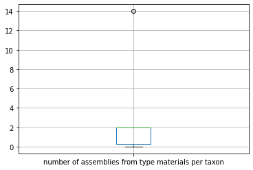
These are just a few examples on how to use a boxplot. See here for more examples: https://pandas.pydata.org/pandas-docs/stable/reference/api/pandas.DataFrame.boxplot.html

pd.__version__

'0.24.2'

Matplotlib

Python has a very useful package known as “matplotlib” (see here: https://matplotlib.org/). It provides a variety of plotting functions and plot types. See some examples here to learn what it can do: https://matplotlib.org/gallery/index.html

These are plots that you wouldn’t be able to plot using Microsoft Excel. R has similar plot functionalities and maybe easier to use than Python libraries. Here, we will explore a few plotting functions. First, you need to import the library before you can use its features.

import matplotlib.pyplot as plt

x = [1, 2, 3, 4, 5, 6, 7, 8, 9, 10]
y = [5, 10, 3, 5, 4, 2, 3, 8, 1, 2]
z = [10, 20, 30, 50, 10, 50, 20, 10, 10, 5]


#plt.scatter(x, y, s=z)
plt.scatter(x, y, c="w", alpha=0.8, edgecolors="r")

<matplotlib.collections.PathCollection at 0x1239bf190>

In this example, I have created a scatter plot with 3 variables: x, y, and z. x contains coordinates of the x-axis, y coordinates of the y-axis, and z the sizes of the scatter dots. If you don’t specify the s in the scatter function it will produce dots with the same size. To learn more about this scatter function, you can type like this:

help(plt.scatter)

Help on function scatter in module matplotlib.pyplot:

scatter(x, y, s=None, c=None, marker=None, cmap=None, norm=None, vmin=None, vmax=None, alpha=None, linewidths=None, verts=<deprecated parameter>, edgecolors=None, *, plotnonfinite=False, data=None, **kwargs)
    A scatter plot of *y* vs. *x* with varying marker size and/or color.

    Parameters
    ----------
    x, y : float or array-like, shape (n, )
        The data positions.

    s : float or array-like, shape (n, ), optional
        The marker size in points**2.
        Default is ``rcParams['lines.markersize'] ** 2``.

    c : array-like or list of colors or color, optional
        The marker colors. Possible values:

        - A scalar or sequence of n numbers to be mapped to colors using
          *cmap* and *norm*.
        - A 2-D array in which the rows are RGB or RGBA.
        - A sequence of colors of length n.
        - A single color format string.

        Note that *c* should not be a single numeric RGB or RGBA sequence
        because that is indistinguishable from an array of values to be
        colormapped. If you want to specify the same RGB or RGBA value for
        all points, use a 2-D array with a single row.  Otherwise, value-
        matching will have precedence in case of a size matching with *x*
        and *y*.

        If you wish to specify a single color for all points
        prefer the *color* keyword argument.

        Defaults to `None`. In that case the marker color is determined
        by the value of *color*, *facecolor* or *facecolors*. In case
        those are not specified or `None`, the marker color is determined
        by the next color of the ``Axes``' current "shape and fill" color
        cycle. This cycle defaults to :rc:`axes.prop_cycle`.

    marker : `~.markers.MarkerStyle`, default: :rc:`scatter.marker`
        The marker style. *marker* can be either an instance of the class
        or the text shorthand for a particular marker.
        See :mod:`matplotlib.markers` for more information about marker
        styles.

    cmap : str or `~matplotlib.colors.Colormap`, default: :rc:`image.cmap`
        A `.Colormap` instance or registered colormap name. *cmap* is only
        used if *c* is an array of floats.

    norm : `~matplotlib.colors.Normalize`, default: None
        If *c* is an array of floats, *norm* is used to scale the color
        data, *c*, in the range 0 to 1, in order to map into the colormap
        *cmap*.
        If *None*, use the default `.colors.Normalize`.

    vmin, vmax : float, default: None
        *vmin* and *vmax* are used in conjunction with the default norm to
        map the color array *c* to the colormap *cmap*. If None, the
        respective min and max of the color array is used.
        It is deprecated to use *vmin*/*vmax* when *norm* is given.

    alpha : float, default: None
        The alpha blending value, between 0 (transparent) and 1 (opaque).

    linewidths : float or array-like, default: :rc:`lines.linewidth`
        The linewidth of the marker edges. Note: The default *edgecolors*
        is 'face'. You may want to change this as well.

    edgecolors : {'face', 'none', *None*} or color or sequence of color, default: :rc:`scatter.edgecolors`
        The edge color of the marker. Possible values:

        - 'face': The edge color will always be the same as the face color.
        - 'none': No patch boundary will be drawn.
        - A color or sequence of colors.

        For non-filled markers, the *edgecolors* kwarg is ignored and
        forced to 'face' internally.

    plotnonfinite : bool, default: False
        Set to plot points with nonfinite *c*, in conjunction with
        `~matplotlib.colors.Colormap.set_bad`.

    Returns
    -------
    `~matplotlib.collections.PathCollection`

    Other Parameters
    ----------------
    **kwargs : `~matplotlib.collections.Collection` properties

    See Also
    --------
    plot : To plot scatter plots when markers are identical in size and
        color.

    Notes
    -----
    * The `.plot` function will be faster for scatterplots where markers
      don't vary in size or color.

    * Any or all of *x*, *y*, *s*, and *c* may be masked arrays, in which
      case all masks will be combined and only unmasked points will be
      plotted.

    * Fundamentally, scatter works with 1-D arrays; *x*, *y*, *s*, and *c*
      may be input as N-D arrays, but within scatter they will be
      flattened. The exception is *c*, which will be flattened only if its
      size matches the size of *x* and *y*.

    .. note::
        In addition to the above described arguments, this function can take
        a *data* keyword argument. If such a *data* argument is given,
        the following arguments can also be string ``s``, which is
        interpreted as ``data[s]`` (unless this raises an exception):
        *x*, *y*, *s*, *linewidths*, *edgecolors*, *c*, *facecolor*, *facecolors*, *color*.

        Objects passed as **data** must support item access (``data[s]``) and
        membership test (``s in data``).

This prints the help document associated with the scatter function from Matplotlib. You can also go to the Matplotlib page to see examples on how to customize your plots.

Seaborn

Another Python package I really like using is known as “Seaborn” and it is designed to visualize statistical data. See here: https://seaborn.pydata.org/

Here, we will try to plot the x, y, and z data we just plotted earlier. First, you need to put the data into a dataframe before you can use Seaborn functions.

import seaborn as sns
import pandas as pd

df1 = pd.DataFrame(
    {'x': x,
     'y': y,
     'z': z}
)

g = sns.relplot(x="x", y="y", size="z", data=df1, color="#5710a3")

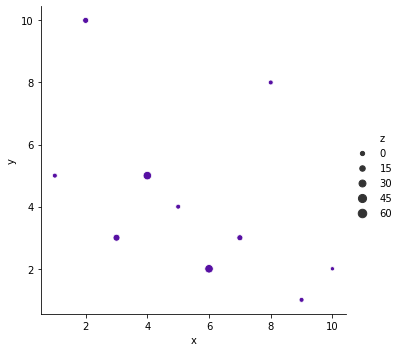
Here, if you look at the code snippet, I am importing both seaborn and pandas to use features provided by these two packages. First, I used Pandas’ DataFrame function to put the list into a dataframe. For this to work, I had to put the list into a dictionary first (see the curly brackets). Then I use Seaborn’s relplot function to create a scatter plot. I provided a custom color code “#5710a3”, which is a hexadecimal code for colors. See here for other options: https://htmlcolorcodes.com/

For additional examples of what Seaborn can do, look here: https://seaborn.pydata.org/examples/index.html

Biopython

Last thing we will go over today is a package known as Biopython. It provides a plethora of useful functions and tools to analyze biological data. There is a vast range of capabilities provided by the library. See here (https://biopython.org/) and here (http://biopython.org/DIST/docs/tutorial/Tutorial.html).

This is my go-to package to analyze biological sequence data. You can browse through the tutorial to see what the package can offer. For example, we can download a genome from NCBI to do some sequence analysis. Download this file (as an example) into your folder where you have this Jupyter lab instance running.

ftp://ftp.ncbi.nlm.nih.gov/genomes/all/GCA/000/006/665/GCA_000006665.1_ASM666v1/GCA_000006665.1_ASM666v1_genomic.gbff.gz

Then unzip the file using gunzip. Now, we can use this unzipped gbff file, which is in Genbank format. First, let’s look at basic statistics of this organism’s genome.

from Bio import SeqIO

records = list(SeqIO.parse("GCA_000006665.1_ASM666v1_genomic.gbff", "genbank"))

print("Found %i records" % len(records))

Found 2 records

First, we are “parsing” the Genbank file and putting the sequence objects into a list named records. It found 2 sequence records. Let’s see what they contain.

records

[SeqRecord(seq=Seq('AGCTTTTCATTCTGACTGCAACGGGCAATATGTCTCTGTGTGGATTAAAAAAAG...TTC', IUPACAmbiguousDNA()), id='AE005174.2', name='AE005174', description='Escherichia coli O157:H7 str. EDL933 genome', dbxrefs=['BioProject:PRJNA259', 'BioSample:SAMN02604092']),
 SeqRecord(seq=Seq('ATGGCAGAGCAAAAACGACCGGTACTGACACTGAAGCGGAAAACGGAAGGAGAG...AGC', IUPACAmbiguousDNA()), id='AF074613.1', name='AF074613', description='Escherichia coli O157:H7 str. EDL933 plasmid pO157, complete sequence', dbxrefs=['BioProject:PRJNA259', 'BioSample:SAMN02604092'])]

for i in records:
    print(i.description)

Escherichia coli O157:H7 str. EDL933 genome
Escherichia coli O157:H7 str. EDL933 plasmid pO157, complete sequence

So this Genbank file contains two sequences from E. coli O157:H7, a pathogenic form of the bacterium that causes food poisonings every year. Let’s take a closer look at the plasmid pO157 to see what genes it contains.

plasmid = records[1]
for f in plasmid.features:
    if f.type == "CDS":
        print(f.qualifiers['locus_tag'][0], f.qualifiers['product'][0])

Z_L7001 fertility inhibition protein (conjugal transfer repressor)
Z_L7002 unknown
Z_L7003 hypothetical protein 15.6 kDa protein in finO 3' region precursor
Z_L7004 putative hemolysin expression modulating protein
Z_L7005 hypothetical protein
Z_L7006 CopB protein (RepA2 protein)
Z_L7007 replication initiation protein
Z_L7008 replication initiation protein
Z_L7009 replication protein
Z_L7010 unknown
Z_L7011 hypothetical protein
Z_L7012 unknown
Z_L7013 transposase (partial)
Z_L7014 hypothetical protein
Z_L7015 transposase
Z_L7016 unknown
Z_L7017 EHEC-catalase/peroxidase
Z_L7018 hypothetical protein
Z_L7019 transposase
Z_L7020 putative exoprotein-precursor
Z_L7021 unknown
Z_L7022 transposase
Z_L7023 hypothetical protein
Z_L7024 regulatory protein
Z_L7025 unknown
Z_L7026 hypothetical protein
Z_L7027 hypothetical protein
Z_L7028 hypothetical protein
Z_L7029 putative acyltransferase
Z_L7030 unknown
Z_L7031 hypothetical protein
Z_L7032 type II secretion protein
Z_L7033 type II secretion protein
Z_L7034 type II secretion protein
Z_L7035 type II secretion protein
Z_L7036 type II secretion protein
Z_L7037 type II secretion protein
Z_L7038 type II secretion protein
Z_L7039 type II secretion protein
Z_L7040 type II secretion protein
Z_L7041 type II secretion protein
Z_L7042 type II secretion protein
Z_L7043 type II secretion protein
Z_L7044 type II secretion protein
Z_L7045 hypothetical protein
Z_L7046 ORFB of IS911
Z_L7047 hemolysin transport protein
Z_L7048 hemolysin toxin protein
Z_L7049 hemolysin transport protein
Z_L7050 hemolysin transport protein
Z_L7051 hypothetical protein
Z_L7052 hypothetical protein
Z_L7053 hypothetical serine-threonine protein kinase
Z_L7054 replication protein
Z_L7055 replication protein
Z_L7056 replication protein
Z_L7057 replication protein
Z_L7058 hypothetical protein
Z_L7059 hypothetical protein
Z_L7060 hypothetical protein
Z_L7061 hypothetical protein
Z_L7062 plasmid maintenance protein
Z_L7063 plasmid maintenance protein
Z_L7064 resolvase (protein d)
Z_L7065 transposase
Z_L7066 hypothetical protein
Z_L7067 Rep protein E1
Z_L7068 plasmid partitioning protein
Z_L7069 plasmid partitioning protein
Z_L7070 hypothetical protein
Z_L7071 unknown
Z_L7072 unknown
Z_L7073 unknown
Z_L7074 hypothetical protein
Z_L7075 unknown
Z_L7076 unknown
Z_L7077 unknown
Z_L7078 unknown
Z_L7079 unknown
Z_L7080 unknown
Z_L7081 unknown
Z_L7082 unknown
Z_L7083 unknown
Z_L7084 single strand binding protein
Z_L7085 hypothetical protein
Z_L7086 hypothetical protein
Z_L7087 putative regulator of SOS induction
Z_L7088 hypothetical protein
Z_L7089 hypothetical protein
Z_L7090 stable plasmid inheritance protein
Z_L7091 putative nickase
Z_L7092 hypothetical protein
Z_L7093 putative transposase
Z_L7094 transposase
Z_L7095 putative cytotoxin
Z_L7096 putative transposase
Z_L7097 hypothetical protein
Z_L7098 DNA helicase
Z_L7099 acetylase for F pilin
Z_L7100 hypothetical protein 31.7 kDa protein in traX-finO intergenic region

Here, what you can see here is that I have listed all the coding sequences within this plasmid and printed their annotations. As you can see, it contains a lot of virulence factors such as “hemolysin toxin protein”, “type II secretion protein”, and “putative cytotoxin”, etc. There are also a bunch of hypothetical and unknown proteins. This is quite typical of microbial genomes. Roughly about 30% of the genes in microbial genomes tend to have no known function.

So this plasmid is the reason this E. coli strain causes food poisoning in humans and animals. In non-pathogenic E. coli strains, you will not find this plasmid. Let’s say if you want to list the coding regions (gene coordinates) of these genes, you can type something like this:

for f in plasmid.features:
    if f.type == "CDS":
        print(f.qualifiers['locus_tag'][0], f.location)

Z_L7001 [0:561](+)
Z_L7002 [697:949](+)
Z_L7003 [1150:1612](+)
Z_L7004 [1657:1867](+)
Z_L7005 [1904:2243](+)
Z_L7006 [2482:2737](+)
Z_L7007 [2972:3047](+)
Z_L7008 [3039:3897](+)
Z_L7009 [4258:4453](+)
Z_L7010 [4809:5094](+)
Z_L7011 [5093:5369](+)
Z_L7012 [5439:5727](-)
Z_L7013 [5754:5976](-)
Z_L7014 [6028:6763](-)
Z_L7015 [6546:7056](-)
Z_L7016 [7040:7280](+)
Z_L7017 [7372:9583](+)
Z_L7018 [9626:10016](+)
Z_L7019 [10173:11061](+)
Z_L7020 [11241:15144](+)
Z_L7021 [15306:15414](-)
Z_L7022 [15608:15881](-)
Z_L7023 [16147:16297](-)
Z_L7024 [16586:16721](+)
Z_L7025 [16881:17055](+)
Z_L7026 [17322:18144](+)
Z_L7027 [18146:19250](+)
Z_L7028 [19339:21061](+)
Z_L7029 [21101:22133](+)
Z_L7030 [22420:22594](+)
Z_L7031 [23015:25712](+)
Z_L7032 [25798:26674](+)
Z_L7033 [26713:28642](+)
Z_L7034 [28641:30147](+)
Z_L7035 [30148:31372](+)
Z_L7036 [31402:31837](+)
Z_L7037 [31833:32388](+)
Z_L7038 [32384:32750](+)
Z_L7039 [32746:33346](+)
Z_L7040 [33342:34320](+)
Z_L7041 [34253:35531](+)
Z_L7042 [35517:36030](+)
Z_L7043 [36087:36921](+)
Z_L7044 [37012:37414](+)
Z_L7045 [37556:37898](+)
Z_L7046 [37942:38764](+)
Z_L7047 [39304:39820](+)
Z_L7048 [39821:42818](+)
Z_L7049 [42867:44988](+)
Z_L7050 [44991:46431](+)
Z_L7051 [46497:46692](+)
Z_L7052 [46721:47006](+)
Z_L7053 [47174:47405](+)
Z_L7054 [47909:48266](+)
Z_L7055 [47954:48272](-)
Z_L7056 [48550:49504](-)
Z_L7057 [49265:49595](+)
Z_L7058 [49935:50172](-)
Z_L7059 [50132:50753](-)
Z_L7060 [50749:51433](-)
Z_L7061 [51488:51683](+)
Z_L7062 [51891:52110](+)
Z_L7063 [52111:52417](+)
Z_L7064 [52417:53224](+)
Z_L7065 [53310:54201](-)
Z_L7066 [54197:54524](-)
Z_L7067 [54668:54824](+)
Z_L7068 [55411:56578](+)
Z_L7069 [56577:57549](+)
Z_L7070 [57933:58206](+)
Z_L7071 [58289:58586](-)
Z_L7072 [58848:60573](+)
Z_L7073 [60649:61552](+)
Z_L7074 [61937:62621](+)
Z_L7075 [62736:63291](+)
Z_L7076 [63336:64113](+)
Z_L7077 [64530:64956](+)
Z_L7078 [65002:65425](+)
Z_L7079 [65582:66113](-)
Z_L7080 [66626:66887](-)
Z_L7081 [66890:68252](+)
Z_L7082 [68298:68862](+)
Z_L7083 [68947:69403](-)
Z_L7084 [69665:70157](+)
Z_L7085 [70186:70447](+)
Z_L7086 [70452:72471](+)
Z_L7087 [72522:72960](+)
Z_L7088 [72956:73718](+)
Z_L7089 [73891:74104](+)
Z_L7090 [73949:74108](+)
Z_L7091 [74289:76263](+)
Z_L7092 [76330:76762](+)
Z_L7093 [77321:77681](-)
Z_L7094 [77862:78273](+)
Z_L7095 [78541:88051](+)
Z_L7096 [88142:88415](+)
Z_L7097 [88341:88845](-)
Z_L7098 [88991:90290](+)
Z_L7099 [90309:91056](+)
Z_L7100 [91114:91975](+)

This prints a list of gene coordinates for the coding sequences in this plasmid and also the coding strands (either plus or minus). You can even draw a genome diagram using Biopython. Here is an example.

from reportlab.lib import colors
from reportlab.lib.units import cm
from Bio.Graphics import GenomeDiagram
from Bio import SeqIO

gd_diagram = GenomeDiagram.Diagram("E. coli plasmid")
gd_track_for_features = gd_diagram.new_track(1, name="Annotated Features")
gd_feature_set = gd_track_for_features.new_set()

for feature in plasmid.features:
    if feature.type != "gene":
        # Exclude this feature
        continue
    if len(gd_feature_set) % 2 == 0:
        color = colors.blue
    else:
        color = colors.lightblue
    gd_feature_set.add_feature(feature, color=color, label=True)

gd_diagram.draw(
    format="linear",
    orientation="landscape",
    pagesize="A4",
    fragments=4,
    start=0,
    end=len(plasmid),
)

gd_diagram.write("plasmid_linear.pdf", "PDF")

This will produce a file named “plasmid_linear.pdf” and will display the genes found in this plasmid in order. You can also create a circular genome diagram like this:

gd_diagram.draw(
    format="circular",
    circular=True,
    pagesize=(20 * cm, 20 * cm),
    start=0,
    end=len(plasmid),
    circle_core=0.7,
)
gd_diagram.write("plasmid_circular.pdf", "PDF")

These produced the PDF files in the same folder as your Jupyter lab instance. Here’s an example of what it looks like:

Again, I am only showing you very briefly what Biopython is capable of doing. Try yourself some examples shown in the tutorials to see what else you can do with it.

Exercise 1 - Write a simple Python script

All the Python examples I have shown here are in the jupyter-lab environment. What if you want to create a Python script and reuse it for some tasks that you frequently need to perform? You can create a standalone python script for that. An example of a very simple standalone python script that can do things we just went over looks like this:

#!/usr/bin/env python

print("Hello, World!")

And you need to save it in a plain text file with extension .py. For example, name it: hello.py.

To run it, you type:

python hello.py

And it simply prints Hello, World! to the screen if you run it in your terminal. Try it and see if you can create a simple script like this one.

Exercise 2 - Write a standalone Python script to parse a Genbank file

I’ve given you an example below and you should save it as something like parse_gb.py.

#!/usr/bin/env python

import sys
from Bio import SeqIO

records = list(SeqIO.parse(sys.argv[1], "genbank"))

for r in records:
    print(r.description)

To run this script with the Genbank file we used as an example, type:

python parse_gb.py GCA_000006665.1_ASM666v1_genomic.gbff

And this script will simply print the description of the records found in this Genbank file. Play around with the different features and functions we’ve gone over to see if you can make a script that you can reuse it over and over again.

What to do when you are lost?

A lot of the time, you can just Google for solutions to a particular problem you are having. But I would highly recommend this website known as “Stackoverflow”. See here: https://stackoverflow.com/

There, you can search for solutions to all coding related questions or problems. There is a good chance that someone may have posted a question you have and someone may have already provided solution(s) to the problem.